10:00

Optimization & MLE
EMSE 6035: Marketing Analytics for Design Decisions
John Paul Helveston
October 21, 2026
Quiz 3
Write your name on the quiz!
Rules:
- Work alone; no outside help of any kind is allowed.
- No calculators, no notes, no books, no computers, no phones.

Week 9: Optimization & MLE
1. Maximum likelihood estimation
2. Optimization (in general)
3. Joins
4. Pilot data cleaning
Week 9: Optimization & MLE
1. Maximum likelihood estimation
2. Optimization (in general)
3. Joins
4. Pilot data cleaning
Computing the likelihood
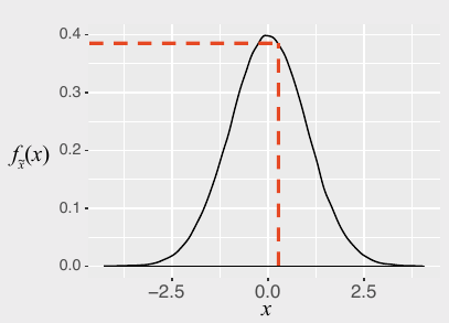
x: an observation
f(x): probability of observing x
Computing the likelihood
x: an observation
f(x): probability of observing x
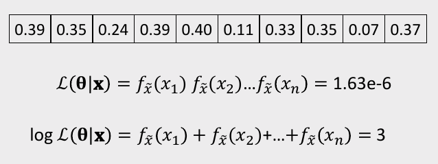
\mathcal{L}(\theta | x): probability that \theta are the true parameters, given that observed x
We want to estimate \theta
We actually compute the log-likelihood
(converts multiplication to addition)
Practice Question 1
Observations - Height of students (inches):
#> [1] 65 69 66 67 68 72 68 69 63 70- Let’s say we know that the height of students, \tilde{x}, in a classroom follows a normal distribution. A professor obtains the above height measurements students in her classroom. What is the log-likelihood that \tilde{x} \sim \mathcal{N} (68, 4)? In other words, compute \ln \mathcal{L} (\mu = 68, \sigma = 4).
- Compute the log-likelihood function using the same standard deviation (\sigma = 4) but with the following different values for the mean, \mu: 66, 67, 68, 69, 70. How do the results compare? Which value for \mu produces the highest log-likelihood?
Week 9: Optimization & MLE
1. Maximum likelihood estimation
2. Optimization (in general)
3. Joins
4. Pilot data cleaning
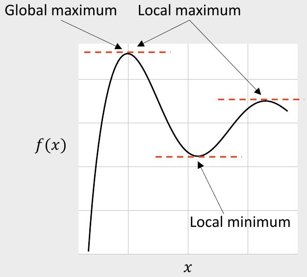
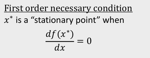
f(x)
Practice Question 2
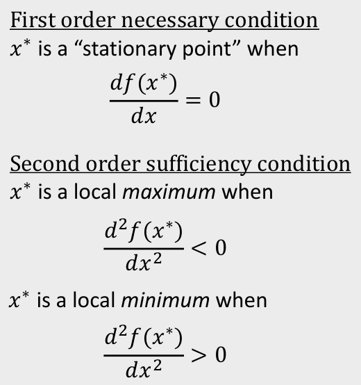
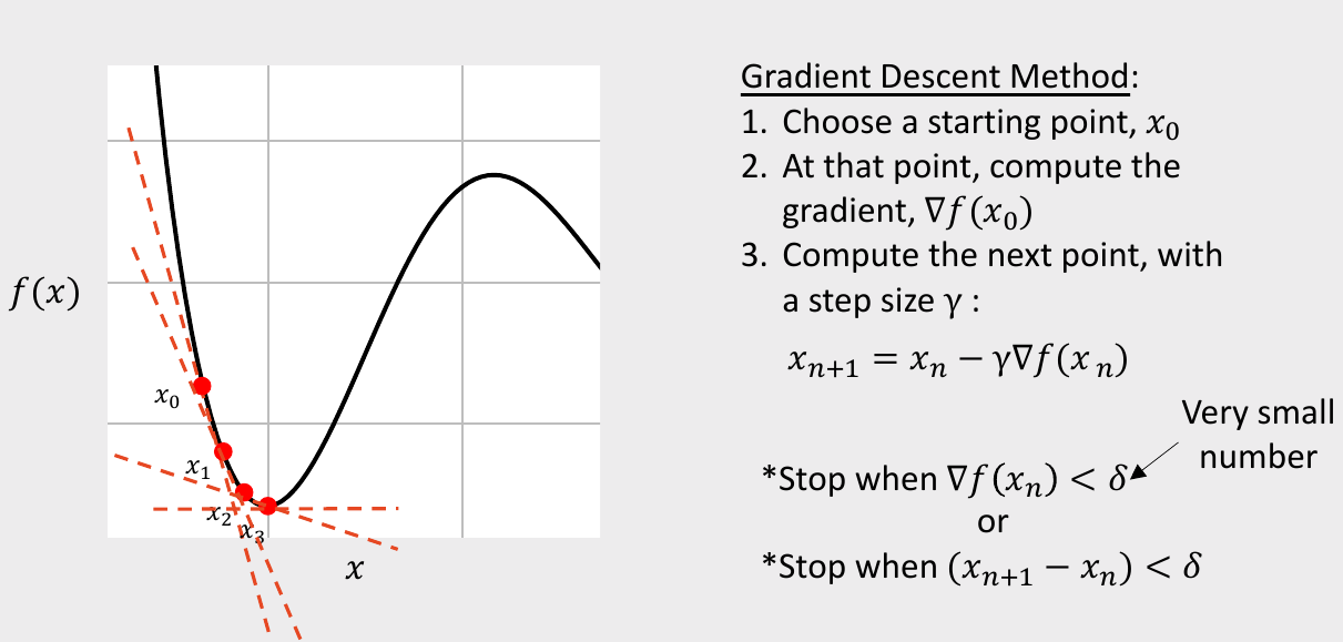
Consider the following function:
f(x) = x^2 - 6x
The gradient is:
\nabla f(x) = 2x - 6
Using the starting point x = 1 and the step size \gamma = 0.3, apply the gradient descent method to compute the next three points in the search algorithm.
Practice Question 3
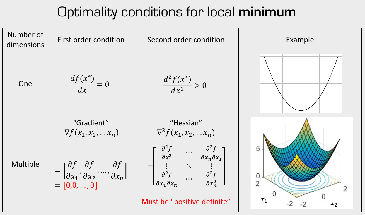
Consider the following function:
f(\underline{x}) = x_1^2 + 4x_2^2
The gradient is:
\nabla f(\underline{x}) = \begin{bmatrix} 2x_1 \\ 8x_2 \end{bmatrix}
Using the starting point \underline{x}_0 = [1, 1] and the step size \gamma = 0.15, apply the gradient descent method to compute the next three points in the search algorithm.
Download the logitr-cars repo from GitHub
Estimating utility models
1. Open the
logitr-cars folder in Positron
2. Open
code/3.1-model-mnl.R
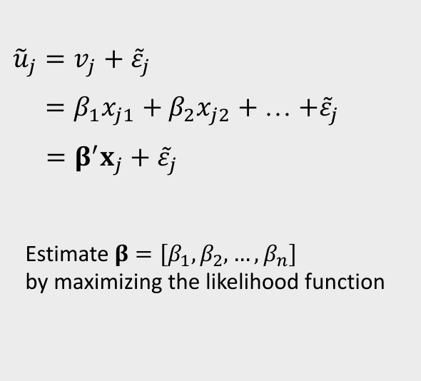
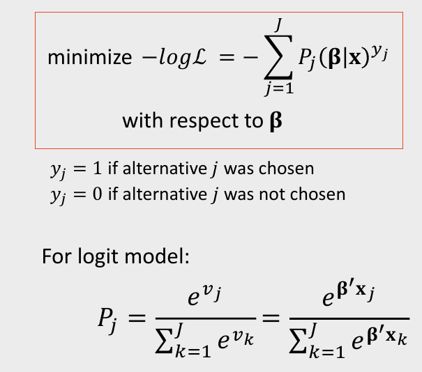
Maximum likelihood estimation
Break
05:00
Week 9: Optimization & MLE
1. Maximum likelihood estimation
2. Optimization (in general)
3. Joins
4. Pilot data cleaning
What’s wrong with this map?
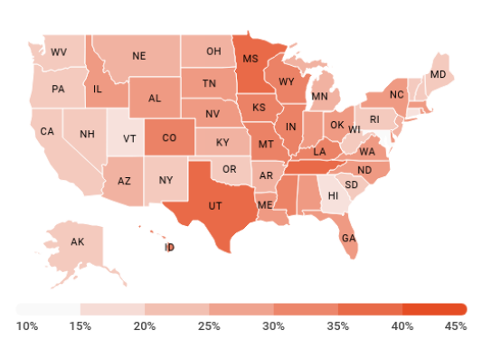
Likely culprit: Merging two columns
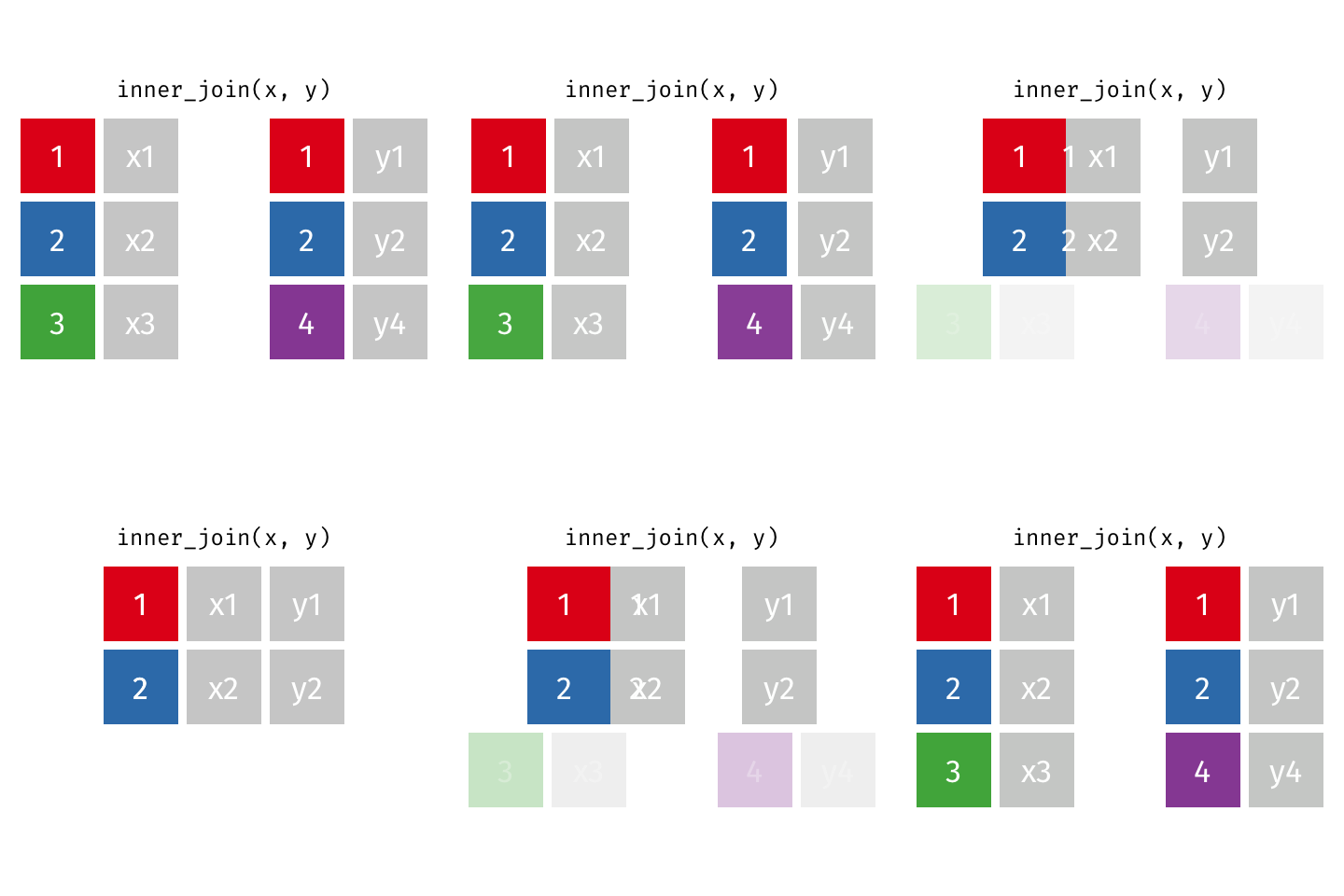
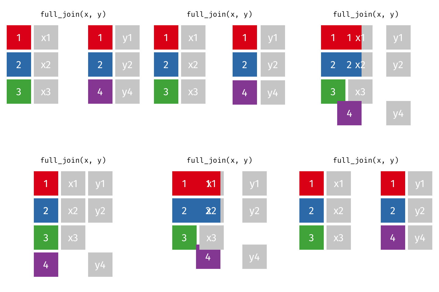
Joins
inner_join()left_join()/right_join()full_join()
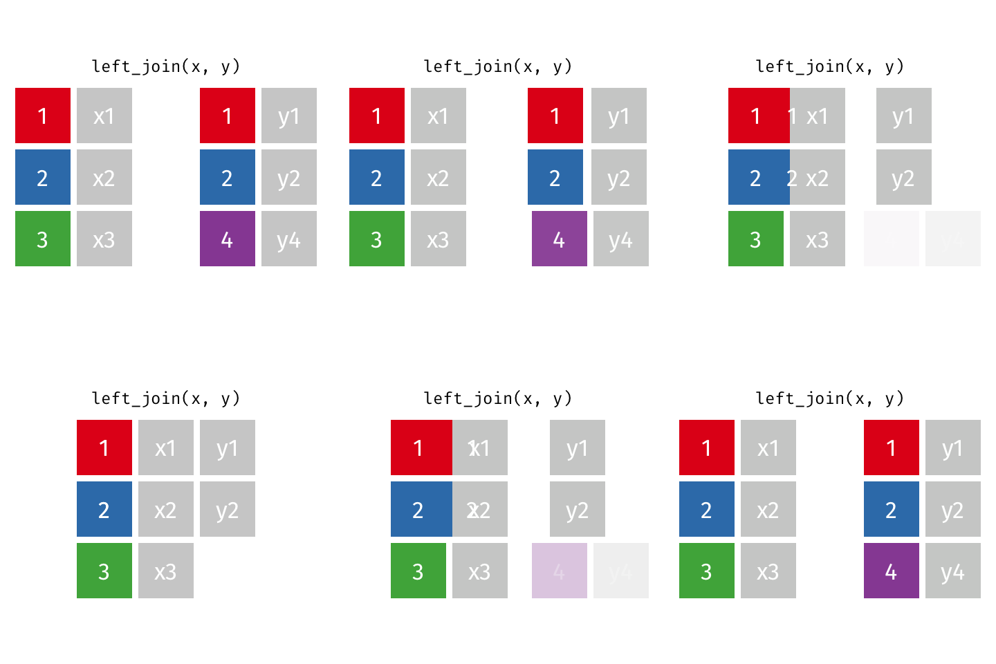
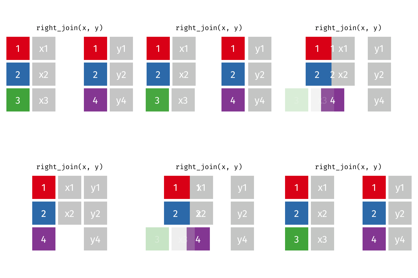
Specify the joining variable name
Specify the joining variable name
If the names differ, use by = c("left_name" = "joining_name")
#> # A tibble: 3 × 2
#>   name  band
#>   <chr> <chr>
#> 1 Mick  Stones
#> 2 John  Beatles
#> 3 Paul BeatlesSpecify the joining variable name
Or just rename the joining variable in a pipe
#> # A tibble: 3 × 2
#>   name  band
#>   <chr> <chr>
#> 1 Mick  Stones
#> 2 John  Beatles
#> 3 Paul Beatles15:00
Your turn
- Create a new data frame called
state_databy joining thestate_abbsandstate_regionsdata frames. The result should be a data frame with variablesstate_name,state_abb, andstate_region. It should look like this:
- Join the
state_datadata frame to thewildlife_impactsdata frame, adding the variablesstate_regionandstate_name.
#> Rows: 56,978
#> Columns: 23
#> $ state_abb             <chr> "FL", "IN", NA, NA, NA, "FL", "FL", NA, NA, "FL", NA, "TX", NA, NA, "NY", NA, NA, "MD", "CA", "AZ", "NC", "TX", NA, NA, "CA", NA, NA, "NM", NA, NA, NA, NA, "CA", "NC", "FL", "FL", "CA", NA, "TX", "CA", "PA", NA, "TX", …
#> $ state_name            <chr> "Florida", "Indiana", NA, NA, NA, "Florida", "Florida", NA, NA, "Florida", NA, "Texas", NA, NA, "New York", NA, NA, "Maryland", "California", "Arizona", "North Carolina", "Texas", NA, NA, "California", NA, NA, "New Mex…
#> $ state_region          <chr> "Southeast", "Corn Belt", NA, NA, NA, "Southeast", "Southeast", NA, NA, "Southeast", NA, "Southern Plains", NA, NA, "Northeast", NA, NA, "Northeast", "Pacific", "Mountain", "Appalachian", "Southern Plains", NA, NA, "Pa…
#> $ incident_date         <dttm> 2018-12-31, 2018-12-29, 2018-12-29, 2018-12-27, 2018-12-27, 2018-12-27, 2018-12-27, 2018-12-26, 2018-12-23, 2018-12-23, 2018-12-23, 2018-12-22, 2018-12-22, 2018-12-22, 2018-12-22, 2018-12-22, 2018-12-21, 2018-12-21, 2…
#> $ airport_id            <chr> "KMIA", "KIND", "ZZZZ", "ZZZZ", "ZZZZ", "KMIA", "KMCO", "ZZZZ", "ZZZZ", "KFLL", "ZZZZ", "KGRK", "ZZZZ", "ZZZZ", "KJFK", "MDPP", "MNMG", "KBWI", "KSMF", "KPHX", "KCLT", "KDFW", "ZZZZ", "ZZZZ", "KSNA", "ZZZZ", "ZZZZ", "K…
#> $ airport               <chr> "MIAMI INTL", "INDIANAPOLIS INTL ARPT", "UNKNOWN", "UNKNOWN", "UNKNOWN", "MIAMI INTL", "ORLANDO INTL", "UNKNOWN", "UNKNOWN", "FORT LAUDERDALE/HOLLYWOOD INTL", "UNKNOWN", "KILLEEN/FT HOOD REGIONAL", "UNKNOWN", "UNKNOWN"…
#> $ operator              <chr> "AMERICAN AIRLINES", "AMERICAN AIRLINES", "AMERICAN AIRLINES", "AMERICAN AIRLINES", "AMERICAN AIRLINES", "AMERICAN AIRLINES", "AMERICAN AIRLINES", "AMERICAN AIRLINES", "AMERICAN AIRLINES", "AMERICAN AIRLINES", "AMERICA…
#> $ atype                 <chr> "B-737-800", "B-737-800", "UNKNOWN", "B-737-900", "B-737-800", "A-319", "A-321", "B-737-800", "A-321", "B-737-800", "B-737-800", "EMB-145", "A-319", "A-319", "B-737-800", "B-737-800", "B-737-800", "A-319", "A-319", "B-…
#> $ type_eng              <chr> "D", "D", NA, "D", "D", "D", "D", "D", "D", "D", "D", "D", "D", "D", "D", "D", "D", "D", "D", "D", "D", "D", "D", "D", "D", "D", "D", "D", NA, "D", "D", "D", "D", "D", "D", "D", "D", "D", "D", "D", "D", "D", "D", "D", …
#> $ species_id            <chr> "UNKBL", "R", "R2004", "N5205", "J2139", "UNKB", "UNKBS", "ZT001", "ZT101", "I1301", "UNKB", "O22", "ZX010", "ZX303", "K5114", "UNKBS", "UNKBS", "UNKB", "J2141", "UNKBS", "ZT101", "UNKB", "UNKB", "ZS009", "UNKB", "UNKB…
#> $ species               <chr> "Unknown bird - large", "Owls", "Short-eared owl", "Southern lapwing", "Lesser scaup", "Unknown bird", "Unknown bird - small", "Eastern meadowlark", "Red-winged blackbird", "Cattle egret", "Unknown bird", "Doves", "Pin…
#> $ damage                <chr> "M?", "N", NA, "M?", "M?", "N", "N", "N", "N", "N", "N", "N", "N", "N", NA, "N", "N", "N", "N", "N", "N", "N", "N", "N", "N", "N", NA, "N", NA, "N", "N", "N", "N", "N", "N", "N", "N", "N", "N", NA, "N", "N", "N", NA, "…
#> $ num_engs              <dbl> 2, 2, NA, 2, 2, 2, 2, 2, 2, 2, 2, 2, 2, 2, 2, 2, 2, 2, 2, 2, 2, 2, 2, 2, 2, 2, 2, 2, NA, 2, 2, 2, 2, 2, 2, 2, 2, 2, 2, 2, 2, 2, 2, 2, 2, 2, 2, NA, 2, 2, 2, 2, 2, 2, 2, 2, 2, 2, 2, 2, 2, 2, 2, 2, 2, 2, 2, 2, 2, 2, 2, 2,…
#> $ incident_month        <dbl> 12, 12, 12, 12, 12, 12, 12, 12, 12, 12, 12, 12, 12, 12, 12, 12, 12, 12, 12, 12, 12, 12, 12, 12, 12, 12, 12, 12, 12, 12, 12, 12, 12, 12, 12, 12, 12, 12, 12, 12, 12, 12, 12, 12, 12, 12, 12, 11, 11, 11, 11, 11, 11, 11, 11…
#> $ incident_year         <dbl> 2018, 2018, 2018, 2018, 2018, 2018, 2018, 2018, 2018, 2018, 2018, 2018, 2018, 2018, 2018, 2018, 2018, 2018, 2018, 2018, 2018, 2018, 2018, 2018, 2018, 2018, 2018, 2018, 2018, 2018, 2018, 2018, 2018, 2018, 2018, 2018, 20…
#> $ time_of_day           <chr> "Day", "Night", NA, NA, NA, "Day", "Night", NA, NA, "Day", "Night", "Day", NA, NA, "Day", "Day", "Day", "Day", "Day", "Night", "Day", "Dawn", NA, NA, "Day", NA, NA, "Day", NA, NA, NA, NA, "Day", "Day", "Day", "Day", "D…
#> $ time                  <dbl> 1207, 2355, NA, NA, NA, 955, 948, NA, NA, 1321, 15, 1612, NA, NA, 905, 1457, 1418, 1628, 627, 2130, 719, 747, NA, NA, 1348, NA, NA, 1305, NA, NA, NA, NA, 1345, 944, 1400, 1415, 1150, 800, 1400, 1505, 1731, NA, NA, 1733…
#> $ height                <dbl> 700, 0, NA, NA, NA, NA, 600, NA, NA, 0, NA, 0, NA, NA, 0, 500, 100, 0, 1000, 4500, 300, NA, NA, NA, NA, NA, NA, 0, NA, NA, NA, NA, 0, NA, 0, 100, 0, 3027, 0, NA, 0, NA, 200, NA, 0, 300, 8, NA, 500, NA, NA, NA, NA, NA, …
#> $ speed                 <dbl> 200, NA, NA, NA, NA, NA, 145, NA, NA, 130, NA, NA, NA, NA, NA, 160, 150, NA, NA, 250, NA, NA, NA, NA, NA, NA, NA, 160, NA, NA, NA, NA, 100, NA, NA, 100, 150, 130, 130, NA, 150, NA, 150, NA, NA, 140, 144, NA, 145, NA, N…
#> $ phase_of_flt          <chr> "Climb", "Landing Roll", NA, NA, NA, "Approach", "Approach", NA, NA, "Take-off run", NA, "Landing Roll", NA, NA, "Landing Roll", "Approach", "Approach", "Take-off run", "Climb", "Climb", "Approach", "Approach", NA, NA,…
#> $ sky                   <chr> "Some Cloud", NA, NA, NA, NA, NA, "Some Cloud", NA, NA, "No Cloud", NA, "Some Cloud", NA, NA, "Some Cloud", "No Cloud", "No Cloud", NA, "No Cloud", "No Cloud", "No Cloud", "Some Cloud", NA, NA, NA, NA, NA, "Some Cloud"…
#> $ precip                <chr> "None", NA, NA, NA, NA, NA, "None", NA, NA, "None", NA, "None", NA, NA, "None", "None", "None", NA, "None", "None", "None", "None", NA, NA, NA, NA, NA, "None", NA, NA, NA, NA, "None", "None", NA, "None", "None", "None"…
#> $ cost_repairs_infl_adj <dbl> NA, NA, NA, NA, NA, NA, NA, NA, NA, NA, NA, NA, NA, NA, NA, NA, NA, NA, NA, NA, NA, NA, NA, NA, NA, NA, NA, NA, NA, NA, NA, NA, NA, NA, NA, NA, NA, NA, NA, NA, NA, NA, NA, NA, NA, NA, NA, NA, NA, NA, NA, NA, NA, NA, NA…
Week 9: Optimization & MLE
1. Maximum likelihood estimation
2. Optimization (in general)
3. Joins
4. Pilot data cleaning
Download the conjoint_buttons template repo
Cleaning surveydown survey data
For the rest of class, work with your team to pull in your pilot survey responses and clean your pilot data.
1. Open the
survey folder in Positron
2. Open
code/2_get_raw_data.R
3. Open
code/3_data_cleaning.R